Cleaning and Filtering SWE Data with process
SWEpy’s process module is built to allow fast access to your temperature brightness files.
It also facilitates the cleaning of missing values and smoothing of messy data.
We can see from the image at the bottom of the page that the SWE curve for a single pixel can be quite messy. This is no suprise considering the nature of passive microwave senors. However, to glean as much useful information as we can from this data, we want to increase the signal to noise ration as much as possible.
Obtaining smoother SWE imagery will allow us to easily derive metrics such as rate of accumulation or melt.
Opening SWE Arrays with get_array
netCDF files are great for storing data, but they aren’t always the easiest to work with. Especially since we store our 19GHz band at a lower resolution than the 37GHz band, we have to downsample one array to match the other anytime we want to find SWE.
In order to save time, get_array looks at metadata of a given file to determine whether to donwsample or not.
This way, with one function call we can extract the temperature brightness and immediatly begin working with our data.
In this example, we will avoid downsampling until we need to so that we can preserve metadata for saving the files later.
tb19 = process.get_array("my_19ghz_file.nc")
tb37 = process.get_array("my_37ghz_file.nc", downsample=False)
Cleaning Erroneous Data Values in TB Arrays
SWEpy employs a simple vectorized forward fill temporally on data values that are unreasonably large or small.
Temperature brigntness data is prone to having sudden extreme values that are clearly an error in data collection or processing. We can see an example of one of these spikes in the figure below:
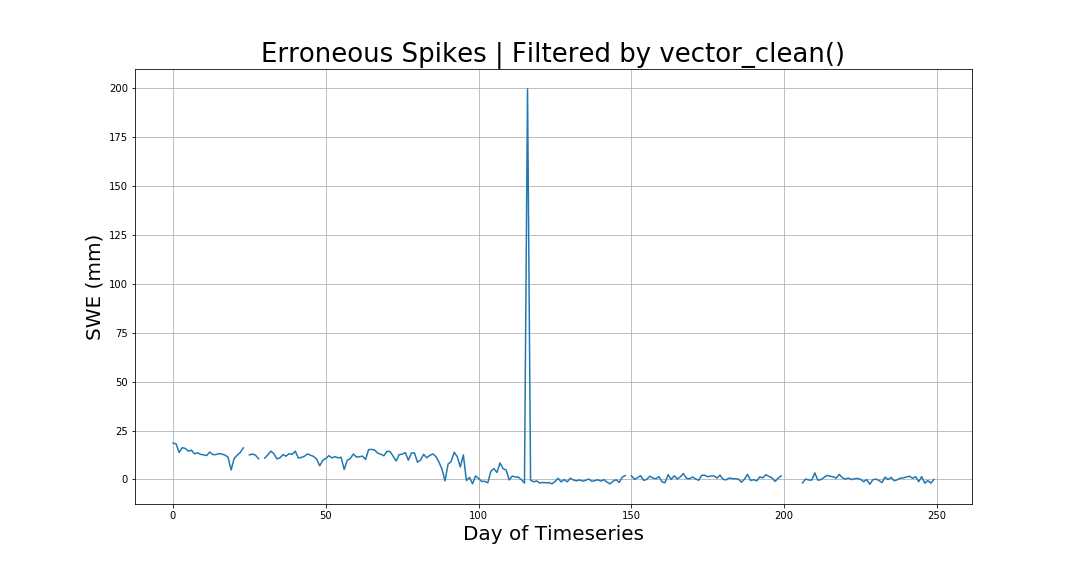
In order to effectivly smooth these arrays, we need to elmininate these spikes!
We use the time vectors because the pixels are quite large (6.25km wide) and doing some sort of nearest neighbor fill often results in weird looking imagery, especially when looking at time series. SWE is very spatially variable, so we want to maintain as much of that spatial information as possible. A single pixel is more like itself the day prior than it is the pixel next to it on the same day.
tb19_clean = process.vector_clean(tb19)
tb37_clean = process.vector_clean(tb37)
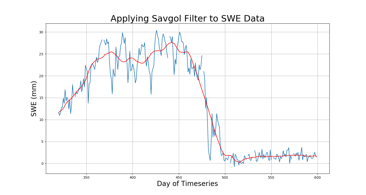
Filtering Data Using a Sav-Gol Filter
As mentioned above, our goal is to increase the signal to noise ratio in the data. We ideally want to smooth temporally since there is more correlation between the same pixel through time than there is between different pixels.
To smooth this data, we use a savitsky-golay filter, which uses the linear least squares method to fit a low-degree polynomial to successive windows of the data.
- NOTE:
apply_filterautomatically uses multiprocessing to spread the problem across all available cores on your machine.If you need a single core solution, use
process.__filter()
import swepy.downsample as down

tb19_filtered = process.apply_fiter(tb19_clean)
tb37_filtered = process.apply_fiter(tb37_clean)

tb37_filtered = down.downsample(tb37_filtered, block_size=(1,2,2), func=np.mean)

swe = process.safe_subtract(tb19_filtered, tb37_filtered)
Finally, we can see the result in the figure below!
Saving TB files Back to netCDF
Now that you have clean temperature brightness files, we can save them back to netCDF to store for later.
The save function works by copying all spatial metadata from the original file, and replacing the original
TB array with our clean version.
NOTE: In order to copy the metadata from the original files, we can’t downsample our tb37 array.
process.save_file("my_19ghz_file.nc", tb19_filtered, "my_19ghz_filtered.nc")
process.save_file("my_37ghz_file.nc", tb37_filtered, "my_37ghz_filtered.nc")
Masking Ocean Pixels from Imagery
Many useful areas of interest contain ocean pixels, which may not be desireable for a given analysis.
A simple solution to solve this is to mask them away. In order to determine which pixels to mask, SWEpy takes a winter day and performs a jenks classification on the image. If there is snow on the ground then sea ice should be the first class since sea ice pixels have lower values than land pixels.
masked_cube = process.mask_ocean_winter(swe_cube, day=0, nclasses=3)